In this article, we’ll see a lot of different functions that one can use to get around their way in MS Excel.
1. Automatically calculating the number of days
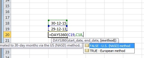
If we have two dates in two different cells, then we can use a function to calculate the number of days between those dates. For instance, we can see the screenshots below, in which we have different dates in cells E18 and E19, and if we wish to calculate the number of days between the two dates then we just enter the formula as ‘=Days360(start date, end date, method)’ It will be better to focus more on start date and end date initially and not on the method.
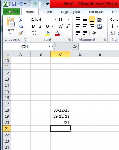
As you can see in the example, if you enter the formula with E4 as the initial day and E5 as the final day, then we get the result as the total number of days between the dates written in E4 and E5.
2. Percent Rank
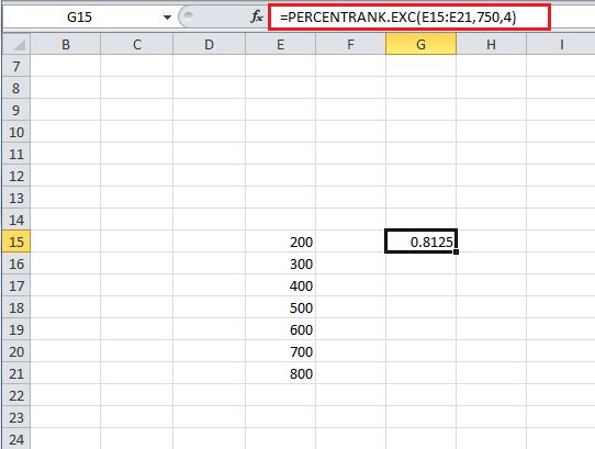
Percent Rank is a function that helps us to find the percent rank of any number with respect to a defined range and also allows us to define the number of significant digits to return the rank for. To use this function, we need to enter ‘=PERCENTRANK(array,x,significance)’ in the cell where we wish to obtain our output. As mentioned, array defines the specified range on the basis of which we are going to rank our number, x is the number for which we wish to find a rank and finally, significance is defined as the number of significant digits to which we wish our rank to be returned. We take the image below as an example for the percent-rank function, we can see that the array/defined range is taken from E15 to E21 and x is taken as 750, the number of significant digits that we have mentioned in this example is 4. Finally the output that we get is equal to 0.8125.
3. Automatically calculating the number of working days (5 days a week)
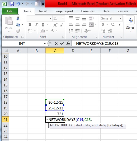
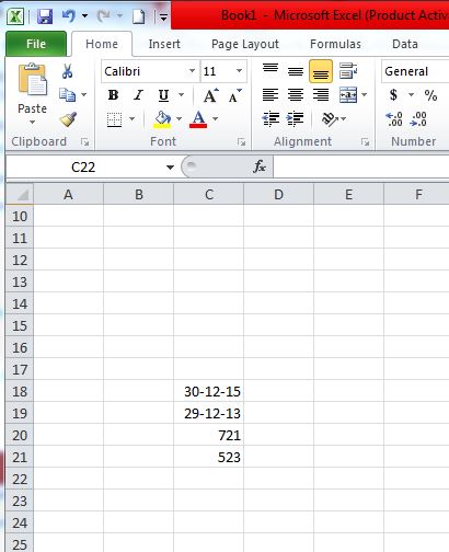
This formula is somewhat similar to the first formula, but this formula is really useful if we wish to find the number of working days between two different dates. We can use this formula by entering ‘=NetworkDays(start date, end date, holidays)’, entering start date and the end date will help the system to remove all the Saturdays and Sundays(and extra holidays, if entered) from the total number of days between those two dates.
As you can see in the example taken, when we enter this networkdays formula in cell C21, then add the dates from cells C18 and C19, then we get the result as 523, as opposed to 721 in C20 that we got by using the formula of calculating the total number of days.
4. Trim
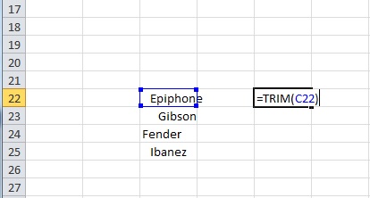
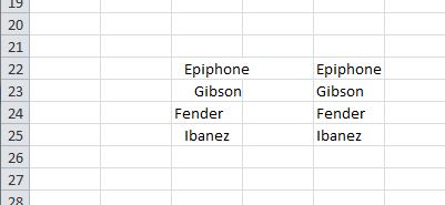
When we copy data from certain places or use tools to import data from the web, we end up having spaces around the data in individual data cells. Excel provides a wonderful formula to take care of this issue, and the formula or function is known as TRIM. So for using trim, we enter ‘=TRIM(cell’s address)’ into the cell where we wish to get our result and then press enter. As can be seen in the example, Trimming C22 (which happens to be the cell with Epiphone written in it) gives us Epiphone without spaces, and same is the case with all the other cells below Epiphone down to Ibanez, as we trim all of them to get a final result without any extra spaces.
5. Percentile
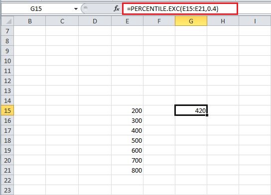
The percentile function helps to return the nth percentile from a set of values. For this, we need to enter ‘=PERCENTILE(array, nth_percentile)’ into a cell where we intend to get our result/output. Here array is the range from which we wish our function to return the nth percentile and as the name suggests, nth percentile is the percentile that we wish to see in our output. The value of percentile can be anywhere between 0 and 1. For example, we can see the image below, in which we have our cell G15, with the function of percentile entered in it, and as we can see the 0.4th percentile in this given set of values, i.e. between E15 and E21 is 420.
6. Concatenate
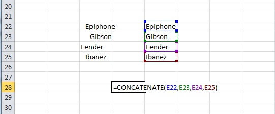
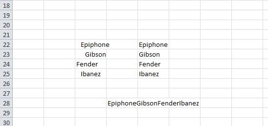
Ever felt like combining the contents of various cells into one single cell? Then excel has got a function just for you, it is called the concatenate function, to use it you just need to enter ‘=Concatenate(Cell 1’s address, Cell 2’s address, Cell 3’s address,.. Cell n’s address)’ and upon pressing enter you’ll see all of your data from the mentioned cells coming into the cell where you entered the concatenation function. For instance, in the example we can see the concatenation of cells E22 to E25 (which happen to be the highlighted cells from Epiphone to Ibanez), and the end result of using the concatenation function turns out to be the concatenation of data from all the selected cells (E22 to E25).
7. Datevalue
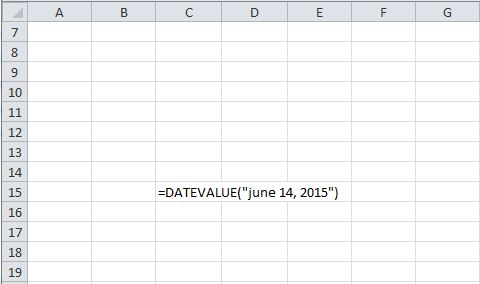
Every date has a value associated with it in Excel; these values can be used for calculation if the need arises. For getting the value of a date, all you need to do is enter ‘=DATEVALUE(“Date”)’ into a cell, and on pressing enter, you’ll see the value that excel provides you corresponding to that particular date.
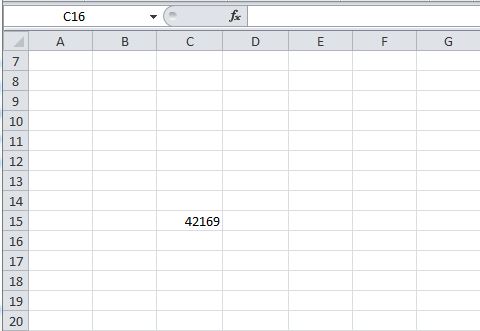
As an example, we have taken the date to be ‘June 14, 2015’, and on using the DATEVALUE function on it, we get a value of 42169.
8. Slope
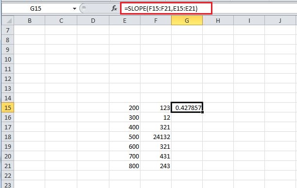
Almost all of us who have studied mathematics or maybe physics to a certain level know what slope is. We all can recall finding slope of a line or a set of points or of some data, using different formulas. When it all comes down to excel, it gets as easy as it can get, excel makes it easy by straightway providing a function for it, it is called the slope function. In this function, we need to enter ‘=SLOPE (known y’s, known x’s)’. Known x and known y are nothing but the x and y coordinates, using which we need to find our slope. So we take a number of x values and an exact same number of y values for this formula, we can do it by selecting all the x values when we are asked to mention the x coordinates in the formula and select all the y values when we are asked to do that. For instance, we can see that in the example below, we have taken the cell G15 and entered the formula ‘=SLOPE (F15:F21, E15:E21)’ and as a result, we get a value of 0.427857 in it. (You can see the formula on the top in front of ‘fx’.
9. Lookup
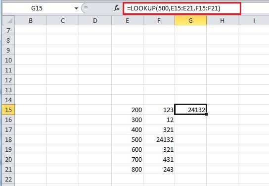
Let us suppose that we have a huge stack of data, and we need to lookup for values corresponding to some other values in the system. For instance, if we have a stack of data with entries in two different columns (let us assume all the entries in first column are related to the entries in second column), for example we can take the value of shares on any particular day, but here shares are marked with numbers instead of their names. So if we were to find the value of a share at a given day, we would use a function known as LOOKUP to straightaway provide us a result, instead of doing a manual search for it. For this formula, we enter ‘=LOOKUP(lookup value, lookup vector, result vector)’, lookup value is the value that we need to look up against(i.e. the name of the share in our example), and the lookup vector is the vector in which our lookup value exists (in our example, lookup vector is the vector containing name of the shares, but we need to remember that here shares are represented by numbers and not by words or alphabets). Finally, the result vector is the one in which we intend to locate the result (in our example, result vector contains the value of shares on a given day). Now if we have a look at the image below, we’ll see the function LOOKUP added in the cell G15, and we take our lookup value as 500(present in the column E), take the lookup vector as the set of values in column E(from E15 to E21), and finally the result vector as the set of values in the column F from F15 to F21.
When we enter this formula, excel looks for the value 500 in lookup vector and then presents the corresponding value from result vector, and hence the result comes out to be 24132.
10. Match Function
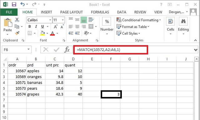
The Microsoft Excel MATCH function searches for a value in an array and returns the relative position of that item. For using the MATCH function, all you need to do is enter ‘=MATCH(value, array, [match_type])’ in the cell where you wish to get the result. Here value signifies the value to be searched in the array, array signifies the range of cells that contain the value that you are searching for and finally match_type is an optional thing that works by having match work in a way in which if match_type =1 the match function finds the largest value less than or equal to value, 0 finds the first value equal to the value and finally -1 will find the smallest value that is greater than or equal to value. As you can see in the example when we add ‘=match(10572,A2:A6,1)’ , you get the value 3
11. IF
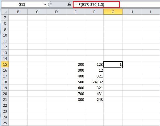
Using an If function would not be alien to anyone who has tried his/her hand on coding, but anyways, one can explain IF function as a conditional function which can provide a specific value if a condition we enter is met, and some other specific value if our condition is not met. For using the IF function, one needs to write ‘=IF (logical test, value if true, value if false)’ in the cell where one intends to obtain his/her result from the IF function. Logical test in this function signifies the logical condition that we wish to use, for instance in the example below we’ll impose a logical condition on a cell E17 by logically testing if the value in it is greater than 370. If the answer to this logical question is true, then a value that we enter in ‘value if true’ in the function, comes out as our answer, otherwise, we’ll get the value entered by us in ‘value if false’.
12. Forecast
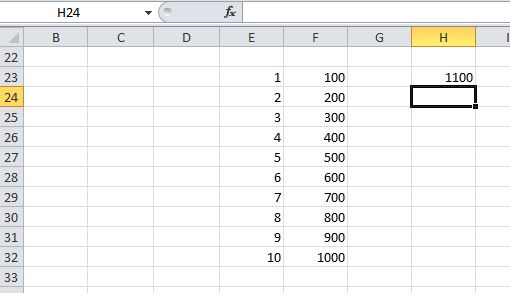
Forecast is a function that helps us to forecast a particular value by looking at the trend in a specified set of data. To use this function, we need to enter ‘=FORECAST(x, known y’s, known x’s)’. Here x and y are two related data sets and known x and known y are the values that are already mentioned. The first x that we write in the function is the one for which we need to find the corresponding value of y. We take a simple example to show the working of this function. In the image below, we can see a simple data set with a pretty easy to decipher relation. So when we mention the easy data set’s values as known x(E23 to E32) and known y(F23 to F32) values, and at the same time we mention the x as 11, in a way we ask our function to forecast the corresponding ‘y’ value when we enter 11 as the value of ‘x’.
As one might have expected, the y value, when x is given a value of 11, turns out to be 1100.
13. AverageIF
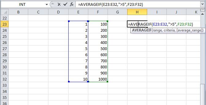
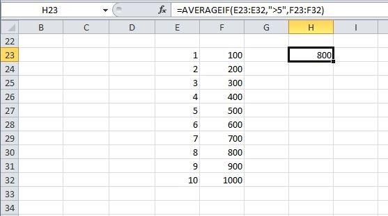
We all know what average is, but excel has a special function which combines the IF function along with the Average function. It is done by averaging only those values that meet a specific criteria mentioned by the If function. For using the IF function, one needs to enter the following into a cell ‘ =AVERAGEIF(range, criteria, average range)’. Here, range defines the set of values on which we’ll be applying the ‘criteria’ mentioned next to it. Criteria helps us to define our If function, we can set a criteria here to use only a specific set of values from the range that we have defined (as we’ll see in the example that follows this description), and finally average range signifies the range of values that we need to average, if we omit the average range part, then our range will be averaged. In the example below, we see that range is taken from E23 to E32, and the criteria is mentioned as ‘>5’, and finally the range is taken from F23 to F32. The result we get is obtained by averaging the values of cells in column F corresponding to the cells in column E that satisfy the criteria (i.e. E28 to E32), and hence we get an average of the values of cells from F28 to F32 (average=800, as can be seen in cell H23).
14. STDEV.P
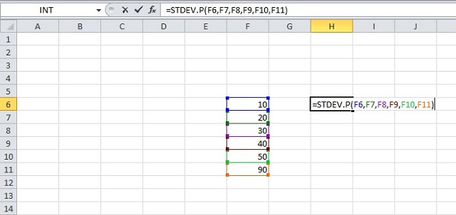
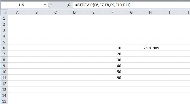
The STDEV.P function in excel returns the standard deviation of a given population. Standard deviation might not be a new term for those who have studied statistics, but it is a long calculative task to measure it manually. Thankfully excel provides a simple way to do it, to use this function, we just need to enter ‘= STDEV.P( number1, [number2, number3,… number])’ here number one is any number or reference to a number and number 2 to number n can be a single number or a set of numbers that we wish to inculcate in the process of calculating standard deviation. A total of 30 values can be entered at a time. An example is shown in the image where we find the standard deviation of a population from F6 to F11.
15. ROUNDUP
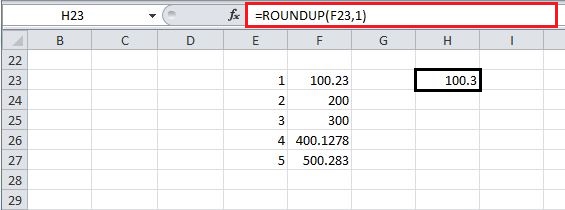
Roundup is a pretty nice tool that helps us to roundup our entries to the places we want. To use this function, we need to enter ‘=ROUNDUP (number, num_digits)’ in a cell and then press enter. Here number signifies the number that we wish to roundup and num_digits represents the number of decimal places to which we wish to roundup our number. As an example, we take H23 in the image below; the function roundup has entries of 100.23 as the number and num_digits as 1. So we get 100.3 as the rounded up value in H23.
SEE ALSO: 15 Cool Excel Tips And Tricks You Should Try We hope this article helped you learn some really helpful Excel functions. If you have any query or suggestion, feel free to let us know in comments.
